On March 15, 2023, EPA released the final “Good Neighbor Plan” (Rule) to require upwind states to reduce emissions of the ozone precursor nitrogen oxide (NOx) from electric generating units (EGUs) and certain stationary industrial sources, in accordance with EPA’s 2015 ozone National Ambient Air Quality Standards (NAAQS). The Rule is effective 60 days after publication in the Federal Register, and litigation challenging the Rule is expected.
In this analysis, we provide an overview of the major regulatory components of the Rule and explore some of the design features affecting the power sector. Specifically, we consider how the Rule looks to balance the need to achieve the statutory-required health and environmental outcomes with the “anticipated continued evolution of the electric power sector toward more efficient and cleaner sources of generation, including as driven by incentives provided by the Infrastructure Investment and Jobs Act as well as the Inflation Reduction Act.”[1]
Why did the EPA issue this rule?
The Clean Air Act (CAA) requires EPA to review and update the ozone NAAQS every five years to protect the public health and welfare.[2] States are responsible for developing and implementing state implementation plans (SIPs) to ensure each attains the applicable ozone NAAQS. CAA section 110(a)(2)(D)(i)(I)–known as the “good neighbor” provision–requires each SIP to include provisions that sufficiently ensure it is not contributing to an air quality concern in another state. Specifically the CAA requires SIPs to “prohibit[ ] . . . any source or other type of emissions activity within the State from emitting any air pollutant in amounts which will—(I) contribute significantly to nonattainment in, or interfere with maintenance by, any other State with respect to any [NAAQS].”[3] If EPA finds that a SIP does not sufficiently reduce interstate air pollution, EPA can issue Federal Implementation Plans (FIPs) to achieve requisite reductions.
In response to prior findings that states’ SIPs did not adequately address their transport of ozone, EPA issued cross-state air pollution FIPs to support downwind states attainment of the 1997 and 2008 ozone NAAQS. The Good Neighbor Plan builds upon those programs to support states attaining the 2015 ozone NAAQS, because EPA during both the Trump and Biden administrations found that certain states’ SIPs inadequately support downwind states’ ozone attainment.[4]
The Rule seeks to achieve the 2015 ozone NAAQS deadlines for “moderate” and “serious” nonattainment by August 3, 2024 and August 3, 2027, respectively. However, EPA also notes that while the prior programs for the 1997 and 2008 ozone NAAQS “successfully drove many EGUs to retrofit post-combustion controls, other EGUs throughout the present geography of linked upwind states continue to operate without such controls and continue to emit at relatively high rates more than 20 years after similar units reduced these emissions.”[5] Thus, EPA includes in this Rule new design features to ensure the Rule achieves the emission reductions consistent with installing and operating control technologies to address good neighbor obligations for the 2015 ozone standard.
How did the EPA develop the Good Neighbor Plan?
The Rule implements FIPs for 23 states and requires those states to reduce emissions from fossil fuel-fired power plants and industrial sources. To determine which states are in the program and what is required for those states, EPA applies the same four-step interstate transport framework that it used in prior interstate air pollution programs to develop the state obligations.[6] Courts have previously upheld EPA’s use of this framework, including most recently on March 3, 2023, when the D.C. Circuit upheld the 2021 Cross-State Air Pollution Rule (CSAPR) Update for the 2008 Ozone NAAQS, rejecting Midwest Ozone Group’s challenge to three of the four steps, arguing that EPA’s technical basis for the rule was arbitrary and capricious.[7]
Through this four-step process, EPA establishes an ozone emissions cap based on installation of available emissions control equipment that can adequately protect public health and welfare. To achieve this result, EPA carries forward previous interstate air pollution cap-and-trade programs for power plants, with several revisions, based on annual emissions budgets that decline over time. EPA sets these caps based on its assumptions about control technology emission rates, timing to install technologies, as well as “current information on the present economic capacity of sources, control-installation vendors, and associated markets for labor and material”, and known retirements.[8] EPA also recognizes that case law in the D.C. Circuit, including in Wisconsin v. EPA,[9] which held that states and EPA must fully address good neighbor obligations as “as expeditiously as practical” and at least by the applicable attainment dates.[10]
However, EPA notes that the installation of certain EGU controls and all non-EGU controls is not possible for the moderate area attainment date of August 3, 2024 and certain sources may not be able to install such technologies by the 2026 ozone season or even the August 3, 2027 serious attainment date.[11] EPA cites “current information on the present economic capacity of sources, control-installation vendors, and associated markets for labor and material” to conclude that a three-year compliance timeframe is not possible for all sources.[12] Therefore, EPA incorporates various compliance flexibilities.
Which sources are covered by the Rule?
Of the 22 states required to reduce emissions from EGUs, 19 were previously included in interstate air pollution programs[13] and three states (Nevada, Utah, and Minnesota) are included for the first time.
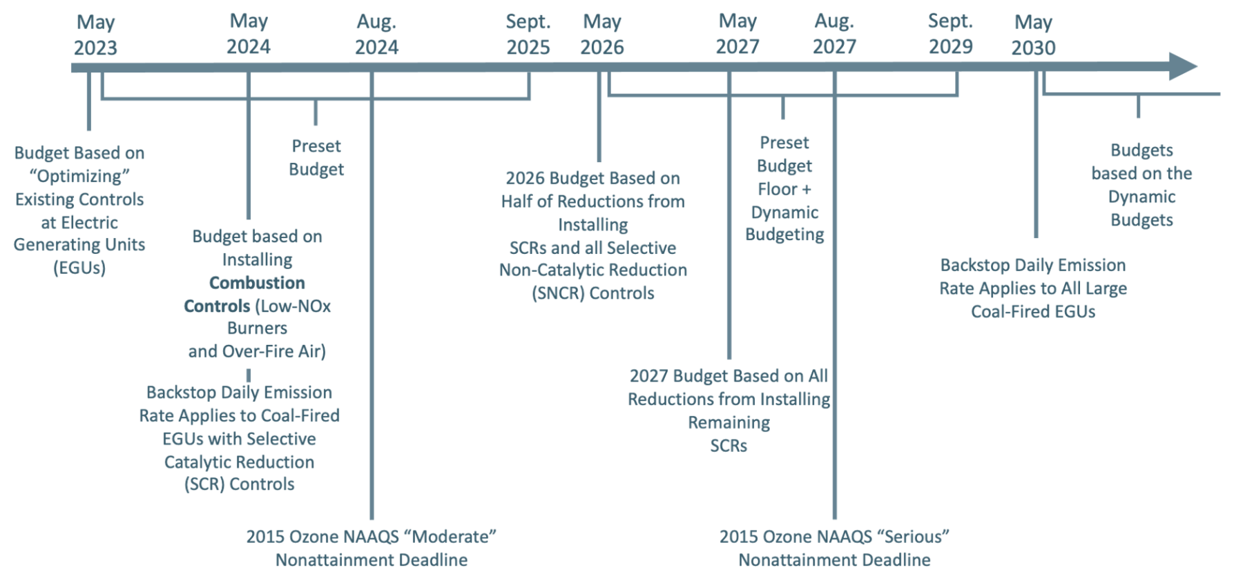
For the 2023 ozone season, which starts May 1, the Rule sets state budgets based on emissions reduced from EGUs optimizing existing post-combustion control and combustion control upgrades. For the remaining ozone seasons, the state budgets are set based on emission reductions achieved through phased installation of “state-of the-art” NOx controls (such as low-NOx burners and over-fire air) beginning in 2024 and new post-combustion controls (selective catalytic reduction [SCR] or selective non-catalytic reduction [SNCR]) starting in the 2026 ozone season.
The Good Neighbor Plan also requires, for the first time, emissions reductions from new and existing non-EGU industrial sources beginning in 2026.[14] This provision covers 20 states,[15] all of which are also covered by the EGU-reduction provisions except for California, in which it only applies to that state’s non-EGUs. It provides a phase-in period for these newly-covered sources by requiring these states to install technology starting in 2026 Ozone Season, and flexibility by including a “process for individual facilities to seek a one year extension, with the possibility of up to two additional years, based on a specific showing of necessity.”[16]
EPA also makes clear that it intends to “expeditiously review the updated air quality modeling and related analyses” to address interstate ozone transport in six additional states in a separate action.[17] These states include: Arizona, Iowa, Kansas, New Mexico, Tennessee, and Wyoming. In the proposed Good Neighbor Plan, EPA found that Oregon and Delaware potentially contributed to interstate pollution. However, in the final rule, EPA rescinded that finding for Delaware and is deferring finalizing a finding for Oregon.
New Design Features for Power Plants
Revised Trading Group
The Rule implements a cap-and-trade program similar to previous interstate air pollution plans, whereby EPA sets states’ emissions budgets that decline over time to support downwind states in achieving the 2015 ozone attainment deadlines. EPA explains that while the trading program “is based on strategies that do not require generation shifting or reduced utilization of EGUs, the sector’s unusual flexibility with respect to how emissions reductions can be achieved makes the flexibility of a trading program particularly useful as a means of lowering the overall costs of obtaining such reductions.”[18]
For states subject to the Good Neighbor Plan, is revising the CSAPR NOx Ozone Season Trading Program by shifting those states in Group 2 into a single Revised Group 3 trading program to “expand the program’s geographic scope and to enhance the program’s ability to ensure favorable environmental outcomes.”[19] To set the preset budgets, EPA used its approach for the CSAPR Update and the Revised CSAPR Update rules[20] and adjusted “the emissions rates and mass emissions to reflect the control stringencies identified as appropriate for EGUs of that type.”[21] EPA states that in “accounting for both the stringency of the rule and known fleet change, the 2026 preset budget is 23 percent lower than the 2025 preset budget; the 2027 preset budget is 20 percent lower than the 2026 preset budget; the 2028 preset budget is 4 percent lower than the 2027 preset budget; and the 2029 preset budget is 8 percent lower than the 2028 preset budget.”[22]
Dynamic Budgets
To maintain the Rule’s selected control stringency and better “reflect future changes in the EGU fleet unknown at the time of the rulemaking,” the Rule uses a combination of “preset” budgets as well as a “dynamic” budgeting procedure.[23] The role and interaction of the preset budget with the dynamic budgeting adjusts depending on the control period, as shown in the table below:
| Control Period | Dynamic Budgeting |
| 2023-2025 | Preset budgets serve as the state emissions budgets with no role for dynamic budgeting |
| 2026-2029 | Preset emission budgets serve as a floor; EPA will only adjust the budget higher if EPA calculates the dynamic budget to be higher than the preset budget due to “heat input patterns across the fleet in service, inclusive of EGU entry and exit” |
| 2030 and later | EPA will publish the state emission budgets based on the dynamic budgets it calculates to reflect all prior retirements and new builds |
For any adjusted budgets starting in 2025, EPA will publish the dynamic budgets and underlying data and calculations in the Federal Register to provide parties the opportunity to seek corrections. EPA also explains that this later period includes “retirements already planned and announced for purposes of compliance with other power sector regulations or fulfillment of utility commitments” that are captured in the preset state budgets and “the likelihood and magnitude of instances where a state’s dynamic budget . . . would be lower than its preset budget for the control period is reduced in this 2026-2029 period relative to control periods further in the future for which retirement plans have not yet been announced.”[24]
Annual Recalibration of Allowance Bank
As part of the design features to “ensure the trading program continues to maintain the . . . emissions control stringency over time”, EPA will also recalibrate the bank of companies’ unused allowances each control period.[25] EPA will adjust the banks by an amount determined as a percentage of the sum of the state emissions budgets for the applicable control period. For the control periods from 2024 through 2029, the target percentage will be 21 percent, and for control periods in 2030 and later years, the target percentage will be 10.5 percent. EPA explains that this recalibration seeks to “prevent allowance surpluses from accumulating and adversely impacting the ability of the trading program in future control periods to maintain the Step 3 emission control stringency.”[26]
The Rule specifies the timing for each recalibration as well as the process of determining the quantity to reduce the bank “to represent a preset percentage of the sum of the state emissions budgets for each control period.”[27] EPA explains that it provided a higher percentage in the 2024 to 2029 control periods to “provide additional support for allowance market liquidity during these years, which both the EPA and commenters view as an important period of generating fleet transition for the power industry.”[28]
Backstop Emissions Rates
The Rule also includes backstop emission limits to “promote more consistent emissions control by individual EGUs” in the trading program.[29] EPA explains that these requirements are designed to ensure that units with controls “have strong incentives to optimize their emissions performance when a state’s assurance level might otherwise be exceeded” and provide greater assurance that emissions controls will deliver “public health and environmental benefits to underserved and overburdened communities”.[30]
The Rule requires large coal plants[31] to meet a daily emissions rate during the applicable ozone season.
- For coal-fired power plants with existing SCR controls the backstop daily rate will begin in the 2024 control period.
- For coal-fired power plants installing SCR controls after 2024, the backstop daily rate will begin in “the earlier of the 2030 control period or the control period after which an SCR is installed”.
Each ton of emissions exceeding such rates–after the first 50 tons–in a control period “will incur a 3-for-1 allowance surrender ratio instead of the usual 1-for-1 allowance surrender ratio.”[32] EPA explains that the 50-ton threshold is a change from the proposal in response to comments concerning the possibility that it could apply to “emissions outside an EGU operator’s control” such as periods of startup and shutdown.[33]
EPA further explains that the backstop daily emission rate does not constitute a mandate for EGUs without existing SCR controls “to install controls or retire but agrees that, as intended, the provisions would create strong incentives to minimize operation of the units unless and until controls are installed, and . . . in some instances retirement and replacement may be a more economically attractive option for the unit’s customers and/or owners than installation of new controls.”[34]
With respect to the second control period, the daily limit only applies to EGUs once they install an SCR, but applies to all units by 2030. EPA explains this change addresses concerns expressed by grid operators and other commenters that application of the daily limit to EGUs without existing SCR controls starting in the 2027 control period would “provide insufficient time for planning and investments needed to facilitate the unit retirements they viewed as likely to be a preferred compliance pathway for some owners.”[35] EPA states that the deferral also addresses concerns that the uncontrolled units need to back up intermittent renewable generation “by ensuring the availability of sufficient time for owners and operators to complete other investments that may be needed to back up renewable generation” after 2029.[36]
Additionally, beginning in 2024, any unit with an installed post-combustion control that contributes to an assurance level exceedance must meet a new, unit-level emissions limitation structured as a prohibition to emit NOx in excess of a defined amount.[37]
The timeline below illustrates when power plants must comply with these regulatory design features:
Electricity Reliability & Cost Considerations
The final rule does not supersede power sector processes that are designed to ensure reliability as the generation resource mix changes. Before an EGU owner decides to retire a unit, the owner must comply with existing processes run by grid operators and other reliability-focused entities. EPA states that the final rule’s “trading program inherently provides ample flexibility to allow such an orderly transition to take place.”[38] EPA further claims that it has “adopted several changes in the final rule to increase flexibility specifically for the early years of the trading program for which commenters have indicated the greatest concerns about electric system reliability.”[39]
EPA also clarifies that the final rule does not require any EGUs “to cease operation” but that “some EGU owners will conclude that . . . retiring a particular EGU and replacing it with cleaner generating capacity is likely to be a more economic option . . . than making substantial investments in new emissions controls at the unit.”[40] Existing regulatory processes may provide “temporary provision of additional revenues to support the EGU’s continued operation until [such] longer-term mitigation measures can be put in place.”[41]
EPA notes that it is “continuing its practice of meeting with the U.S. Department of Energy and the Federal Energy Regulatory Commission to maintain mutual awareness of how federal actions and programs intersect with the industry’s responsibility to maintain electric reliability,” and highlights its recently signed Joint Memorandum on Interagency Communication and Consultation on Electric Reliability.
EPA’s Regulatory Impact Analysis projects that by 2030 this Rule will result in the following changes to the US electric generation resources:
- 232 EGUs fully operating existing SCRs that did not do so in 2019;
- 39 EGUs fully operating existing SNCRs;
- 9 EGUs installing “state-of-the-art combustion controls”;
- 8 GW of “SCR retrofit at coal plants”; and
- 14 GW of additional coal retirements nationwide (a 13 percent reduction of national coal capacity) relative to the baseline.[42]
For 2024 to 2026, EPA estimates that the Rule will lead to a 4 percent reduction in coal fired electricity generation, and a 2 percent and 1 percent increase in natural gas-fired and renewable electricity generation, respectively.[43] The table below lists EPA’s estimated regional electricity rate impacts:
Average Retail Electricity Price Impact (by Region for the Baseline and the Regulatory Control Alternatives, 2030)[44]
| NERC/ISO Subregion | Geographic Region | Final Rule Percent Change from Baseline |
| Texas Reliability Entity | Texas | 5% |
| Midcontinent ISO/South | Mississippi Delta | 2% |
| NPCC/Upstate NY | Upstate New York | 2% |
| PJM/East | Mid-Atlantic | 2% |
| Midcontinent ISO/Central | Middle Mississippi Valley | 1% |
| NPCC/NYC & Long Island | Metropolitan New York | 1% |
| PJM/West | Ohio Valley | 1% |
| PJM/Dominion | Virginia | 1% |
| SERC Reliability Corporation/ Central | Tennessee Valley | 1% |
| Southwest Power Pool/South | Southern Great Plains | 1% |
| Southwest Power Pool/Central | Central Great Plains | 1% |
| WECC/CA North | Northern California | 1% |
| WECC/Basin | Great Basin | 1% |
| Southwest Power Pool/North | Northern Great Plains | -1% |
| Other 11 Subregions | 0% | |
| National | 1% | |
SIP Disapprovals
In accordance with the CAA, EPA must formally find states’ SIPs deficient before it must issue the Good Neighbor Plan FIP. In 2019, the EPA during the Trump administration found several states’ interstate ozone transport provisions deficient, including the Pennsylvania and Virginia SIPs.[45] In 2021, President Biden directed EPA to review other SIPs, and on February 13, 2023 EPA disapproved 21 states’ SIPs. In response, several states challenged this disapproval in their respective jurisdictions’ federal court of appeals, and some filed motions to stay EPA’s SIP disapprovals.[46]
For example, on March 7, 2023, Utah filed a motion for stay, arguing that in disapproving Utah’s SIP, EPA “exceeded its authority by using a policy preference as the standard for determining acceptability of Utah’s SIP, rather than conducting an objective assessment of whether Utah’s SIP meets CAA applicable requirements” and its decision-making was arbitrary and capricious in approving certain SIPs and rejecting others.[47] Utah argues that “EPA’s Final Rule will result in EPA’s imminent imposition of its Proposed Transport FIP, which requires sources in Utah to install costly emission control technologies, despite UDAQ’s findings that such controls are unnecessary” and these “imminent costs of compliance will be borne by Utah’s citizens through increased electric bills and will raise the prospect that power plants will be shuttered, severely compromising the reliability of Utah’s power supply.”[48] In response, EPA filed motions arguing that these challenges are “nationally applicable” and should therefore be heard in the DC Circuit.
It will be important to watch this litigation and its impact on implementation of the Good Neighbor Plan Rule. Regardless of the outcomes, these states still retain flexibility as EPA notes in the Rule that “[a]t any time after the effective date of this rule, states may submit a Good Neighbor SIP to replace the FIP requirements contained in this rule, subject to EPA approval under CAA section 110(a).”[49]
Next Steps
We will track the SIP disapproval litigation and other developments for this rule on our Air Transport Rules History Regulatory Tracker. We will also analyze other final and proposed rules that EPA expects to issue this spring, and how they may impact the power sector here: Power Plant Regulations.
[1] Good Neighbor Plan Rule, p. 379.
[2] 42 U.S.C. § 7409(d)(1).
[3] 42 U.S.C. § 7410(a)(2)(D)(i)(I).
[4] EPA is currently reviewing the Ozone NAAQS, for more information see our Ozone NAAQS Regulatory Tracker.
[5] Good Neighbor Plan Rule, p. 26.
[6] EPA explains that the 4-step interstate transport framework requires the following: (1) identifying downwind receptors that are expected to have problems attaining or maintaining the NAAQS; (2) determining which upwind states contribute to these identified problems in amounts sufficient to “link” them to the downwind air quality problems (i.e., above a contribution threshold of 1 percent of the NAAQS); (3) for states linked to downwind air quality problems, identifying upwind emissions that significantly contribute to downwind nonattainment or interfere with downwind maintenance of the NAAQS through a multifactor analysis; and (4) for states that are found to have emissions that significantly contribute to nonattainment or interfere with maintenance of the NAAQS in downwind areas, implementing the necessary emissions reductions through enforceable measures. Id. at 22.
[7] Midwest Ozone Group v. EPA, 61 F.4th 187 (D.C. Cir. 2023).
[8] Good Neighbor Plan Rule, p. 354.
[9] Wisconsin v. EPA, 938 F.3d 303, 313-14 (D.C. Cir. 2019) (citing North Carolina v. EPA, 531 F.3d 896, 911-13 (D.C. Cir. 2008).
[10] Good Neighbor Plan Rule, p. 129.
[11] Id. at 353.
[12] Id. at 354.
[13] Alabama, Arkansas, Illinois, Indiana, Kentucky, Louisiana, Maryland, Michigan, Minnesota, Mississippi, Missouri, Nevada, New Jersey, New York, Ohio, Oklahoma, Pennsylvania, Texas, Utah, Virginia, West Virginia, and Wisconsin.
[14] These sources include: Reciprocating internal combustion engines in Pipeline Transportation of Natural Gas; kilns in Cement and Cement Product Manufacturing; reheat furnaces in Iron and Steel Mills and Ferroalloy Manufacturing; furnaces in Glass and Glass Product Manufacturing; boilers in Iron and Steel Mills and Ferroalloy Manufacturing, Metal Ore Mining, Basic Chemical Manufacturing, Petroleum and Coal Products Manufacturing, and Pulp, Paper, and Paperboard Mills; and combustors and incinerators in Solid Waste Combustors and Incinerators.
[15] Arkansas, California, Illinois, Indiana, Kentucky, Louisiana, Maryland, Michigan, Mississippi, Missouri, Nevada, New Jersey, New York, Ohio, Oklahoma, Pennsylvania, Texas, Utah, Virginia, and West Virginia.
[16] Good Neighbor Plan Rule, p. 15.
[17] Id. at 19.
[18] Id. at 367.
[19] Id. at 366.
[20] Id. at 433-34.
[21] Id. at 434.
[22] Id. at 33.
[23] EPA explains that “[d]ynamic budgets are a product of the formula promulgated in this action applied to a rolling three-year average of reported heat input data at the state level and a rolling highest-three-of-five-year average of reported heat input data at the unit level.” Id. at 427.
[24] Id. at 430.
[25] Id. at 334.
[26] Id. at 461.
[27] Id. at 370.
[28] Id. at 464.
[29] Id. at 371.
[30] Id. at 372.
[31] Coal-fired steam units serving generators with nameplate capacity greater than or equal to 100 MW in covered states, except circulating fluidized bed units.
[32] EPA explains how these will be calculated: “For each day of the control period where the unit’s average emissions rate for that day was higher than 0.14 lb/mmBtu, the owner or operator will compute what the unit’s reported emissions on that day would have been (given the unit’s reported heat input for the day) at an emissions rate of 0.14 lb/mmBtu. The difference between the unit’s emissions for the day as actually reported and the emissions that would have been reported if the unit’s emissions rate was 0.14 lb/mmBtu is the unit’s daily exceedance. The amount of emissions subject to the 3-for-1 surrender ratio for the control period is the sum of the unit’s daily exceedances for all days of the control period minus 50 tons (but not less than zero).” Good Neighbor Plan Rule, p. 474.
[33] Id. at 476.
[34] Id. at 490.
[35] Id. at 491.
[36] Id. at 493-94.
[37] Id. at 498.
[38] Id. at 405.
[39] Id.
[40] Id. at 404.
[41] Id. at 405.
[42] Regulatory Impact Analysis, p. 27, 165.
[43] Good Neighbor Plan Rule, p. 703.
[44] Regulatory Impact Analysis, p. 168, Table 4-17.
[45] On November 22, 2019 EPA issued a final rule finding that seven states (Maine, New Mexico, Pennsylvania, Rhode Island, South Dakota, Utah, and Virginia) failed to submit complete state implementation plans to limit interstate pollution that affects downwind states’ ability to meet the 2015 ozone NAAQS.
[46] See, e.g., Texas v. EPA, Case No. 23-60069 (5th Cir. Feb 14, 2023); Mississippi, et al. v. EPA, Case No. 23-60069 (5th Cir. Mar. 16, 2023); Utah v. EPA, Case No. 23-9509 (10th Cir. Feb 13, 2023); Oklahoma Gas & Electric Co. v. EPA, Case No. 23-9521 (10th Cir. Mar 16, 2023); Arkansas, et al v. EPA, Docket No. 23-01320 (8th Cir. Feb 16, 2023); Kentucky v. EPA, Case No. 23-3216 (6th Cir. Mar. 13, 2023).
[47] Motion for Stay at 14, Utah v. EPA, Case No. 23-9509 (10th Cir.).
[48] Id. at 23-25 & 2.
[49] Good Neighbor Plan Rule, p. 18.